PV Array geometry introduction

In this section, we will learn how to:

• create a 2D PV array geometry with PV rows at identical heights, tilt angles, and with identical widths

• plot that PV array

• calculate the inter-row direct shading, and get the length of the shadows on the PV rows

• understand what timeseries geometries are, including ts_pvrows and ts_ground

Imports and settings

# Import external libraries
import matplotlib.pyplot as plt

# Settings
%matplotlib inline

Prepare PV array parameters

pvarray_parameters = {
    'n_pvrows': 4,            # number of pv rows
    'pvrow_height': 1,        # height of pvrows (measured at center / torque tube)
    'pvrow_width': 1,         # width of pvrows
    'axis_azimuth': 0.,       # azimuth angle of rotation axis
    'surface_tilt': 20.,      # tilt of the pv rows
    'surface_azimuth': 90.,   # azimuth of the pv rows front surface
    'solar_zenith': 40.,      # solar zenith angle
    'solar_azimuth': 150.,    # solar azimuth angle
    'gcr': 0.5,               # ground coverage ratio
}

Create a PV array and its shadows

Import the OrderedPVArray class and create a transformed PV array object using the parameters above

from pvfactors.geometry import OrderedPVArray

pvarray = OrderedPVArray.fit_from_dict_of_scalars(pvarray_parameters)

Plot the PV array.

Note: the index 0 is passed to the plotting method. We’re explaining why a little later in this tutorial.

# Plot pvarray shapely geometries
f, ax = plt.subplots(figsize=(10, 3))
pvarray.plot_at_idx(0, ax)
plt.show()

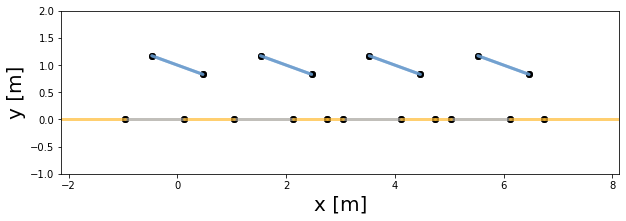
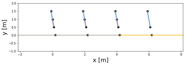
As we can see in the plot above: - the blue lines represent the PV rows - the gray lines represent the shadows cast by the PV rows on the ground from direct light - the yellow lines represent the ground areas that don’t get any direct shading - there are additional points on the ground that may seem out of place: but they are called “cut points” and are necessary to calculate view factors. For instance, if you take the cut point located between the second and third shadows (counting from the left), it marks the point after which the leftmost PV row’s back side is not able to see the ground anymore

Situation with direct shading

We can also create situations where direct shading happens either on the front or back surface of the PV rows.

# New configuration with direct shading
pvarray_parameters.update({'surface_tilt': 80., 'solar_zenith': 75., 'solar_azimuth': 90.})

pvarray_parameters

{'n_pvrows': 4,
 'pvrow_height': 1,
 'pvrow_width': 1,
 'axis_azimuth': 0.0,
 'surface_tilt': 80.0,
 'surface_azimuth': 90.0,
 'solar_zenith': 75.0,
 'solar_azimuth': 90.0,
 'gcr': 0.5}

# Create new PV array
pvarray_w_direct_shading = OrderedPVArray.fit_from_dict_of_scalars(pvarray_parameters)

# Plot pvarray shapely geometries
f, ax = plt.subplots(figsize=(10, 3))
pvarray_w_direct_shading.plot_at_idx(0, ax)
plt.show()

We can now see on the plot above that some inter-row shading is happening in the PV array.

It is also very easy to obtain the shadow length on the front surface of the shaded PV rows.

# Shaded length on first pv row (leftmost)
l = pvarray_w_direct_shading.ts_pvrows[0].front.shaded_length
print("Shaded length on front surface of leftmost PV row: %.2f m" % l)

Shaded length on front surface of leftmost PV row: 0.48 m

# Shaded length on last pv row (rightmost)
l = pvarray_w_direct_shading.ts_pvrows[-1].front.shaded_length
print("Shaded length on front surface of rightmost PV row: %.2f m" %l)

Shaded length on front surface of rightmost PV row: 0.00 m

As we can see, the rightmost PV row is not shaded at all.

What are timeseries geometries?

It is important to note that the two most important attributes of the PV array object are ts_pvrows and ts_ground. These contain what we call “timeseries geometries”, which are objects that represent the geometry of the PV rows and the ground for all timestamps of the simulation.

For instance here, we can look at the coordinates of the front illuminated timeseries surface of the leftmost PV row.

front_illum_ts_surface = pvarray_w_direct_shading.ts_pvrows[0].front.list_segments[0].illum.list_ts_surfaces[0]

coords = front_illum_ts_surface.coords
print("Coords: {}".format(coords))

Coords: [[[ 0.00340618]
  [ 0.98068262]]

 [[-0.08682409]
  [ 1.49240388]]]

These are the timeseries line coordinates of the surface, and it is made out of two timeseries point coordinates, b1 and b2 (“b” for boundary).

b1 = coords.b1
b2 = coords.b2
print("b1 coords: {}".format(b1))

b1 coords: [[0.00340618]
 [0.98068262]]

Each timeseries point is also made of x and y timeseries coordinates, which are just numpy arrays.

print("x coords of b1: {}".format(b1.x))
print("y coords of b1: {}".format(b1.y))

x coords of b1: [0.00340618]
y coords of b1: [0.98068262]

The x and y coordinates will be numpy arrays of all the values the coordinates take for all the simulation timestamps, as calculated at fit() time of the PV array object. This also explain why we needed to specify the index 0 when plotting the PV array: this was to select the coordinates for the first (and only) timestamp.