Run full simulations in parallel

In this section, we will learn how to:

• run full timeseries simulations in parallel (with multiprocessing) using the run_parallel_engine() function

Note: for a better understanding, it might help to read the previous tutorial section on running full timeseries simulations sequentially before going through the following

Imports and settings

# Import external libraries
import os
import numpy as np
import matplotlib.pyplot as plt
from datetime import datetime
import pandas as pd
import warnings

# Settings
%matplotlib inline
np.set_printoptions(precision=3, linewidth=300)
warnings.filterwarnings('ignore')
# Paths
LOCAL_DIR = os.getcwd()
DATA_DIR = os.path.join(LOCAL_DIR, 'data')
filepath = os.path.join(DATA_DIR, 'test_df_inputs_MET_clearsky_tucson.csv')

Get timeseries inputs

def export_data(fp):
    tz = 'US/Arizona'
    df = pd.read_csv(fp, index_col=0)
    df.index = pd.DatetimeIndex(df.index).tz_convert(tz)
    return df

df = export_data(filepath)
df_inputs = df.iloc[:48, :]

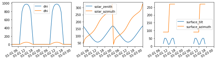
# Plot the data
f, (ax1, ax2, ax3) = plt.subplots(1, 3, figsize=(12, 3))
df_inputs[['dni', 'dhi']].plot(ax=ax1)
df_inputs[['solar_zenith', 'solar_azimuth']].plot(ax=ax2)
df_inputs[['surface_tilt', 'surface_azimuth']].plot(ax=ax3)
plt.show()

# Use a fixed albedo
albedo = 0.2

Prepare PV array parameters

pvarray_parameters = {
    'n_pvrows': 3,            # number of pv rows
    'pvrow_height': 1,        # height of pvrows (measured at center / torque tube)
    'pvrow_width': 1,         # width of pvrows
    'axis_azimuth': 0.,       # azimuth angle of rotation axis
    'gcr': 0.4,               # ground coverage ratio
    'rho_front_pvrow': 0.01,  # pv row front surface reflectivity
    'rho_back_pvrow': 0.03    # pv row back surface reflectivity
}

Run simulations in parallel with run_parallel_engine()

Running full mode timeseries simulations in parallel is done using the run_parallel_engine().

In the previous tutorial section on running timeseries simulations, we showed that a function needed to be passed in order to build a report out of the timeseries simulation.

For the parallel mode, it will not be very different but we will need to pass a class (or an object) instead. The reason is that python multiprocessing uses pickling to run different processes, but python functions cannot be pickled, so a class or an object with the necessary methods needs to be passed instead in order to build a report.

An example of a report building class is provided in the report.py module of the pvfactors package.

# Choose the number of workers
n_processes = 3

# import function to run simulations in parallel
from pvfactors.run import run_parallel_engine
# import the report building class for the simulation run
from pvfactors.report import ExampleReportBuilder

# run simulations in parallel mode
report = run_parallel_engine(ExampleReportBuilder, pvarray_parameters, df_inputs.index,
                            df_inputs.dni, df_inputs.dhi,
                            df_inputs.solar_zenith, df_inputs.solar_azimuth,
                            df_inputs.surface_tilt, df_inputs.surface_azimuth,
                            albedo, n_processes=n_processes)

# make a dataframe out of the report
df_report = pd.DataFrame(report, index=df_inputs.index)
df_report.iloc[6:11, :]

INFO:pvfactors.run:Parallel calculation elapsed time: 0.19188380241394043 sec

	qinc_front	qinc_back	iso_front	iso_back
2019-01-01 07:00:00-07:00	NaN	NaN	NaN	NaN
2019-01-01 08:00:00-07:00	117.632919	9.703464	5.070103	0.076232
2019-01-01 09:00:00-07:00	587.344197	4.906038	12.087407	2.150237
2019-01-01 10:00:00-07:00	685.115436	33.478098	17.516188	3.115967
2019-01-01 11:00:00-07:00	652.526254	52.534503	24.250780	1.697046

f, ax = plt.subplots(1, 2, figsize=(10, 3))
df_report[['qinc_front', 'qinc_back']].plot(ax=ax[0])
df_report[['iso_front', 'iso_back']].plot(ax=ax[1])
plt.show()

The results above are consistent with running the simulations without parallel model (this is also tested in the package).

Building a report for parallel mode

For parallel simulations, a class (or object) that builds the report needs to be specified, otherwise nothing will be returned by the simulation.

Here is an example of a report building class that will return the total incident irradiance ('qinc') on the back surface of the rightmost PV row. A good way to get started building the reporting class is to use the example provided in the report.py module of the pvfactors package.

Another important action of the class is to merge the different reports resulting from the parallel simulations: since the users decide how the reports are built, the users are also responsible for specifying how to merge the reports after a parallel run.

The static method that builds the reports needs to be named build(report, pvarray).

And the static method that merges the reports needs to be named merge(reports).

class NewReportBuilder(object):
    """A class is required to build reports when running calculations with
    multiprocessing because of python constraints"""

    @staticmethod
    def build(pvarray):
        # Return back side qinc of rightmost PV row
        return {'total_inc_back': pvarray.ts_pvrows[1].back.get_param_weighted('qinc').tolist()}

    @staticmethod
    def merge(reports):
        """Works for dictionary reports"""
        report = reports[0]
        # Merge other reports
        keys_report = list(reports[0].keys())
        for other_report in reports[1:]:
            for key in keys_report:
                report[key] += other_report[key]
        return report

# run simulations in parallel mode using the new reporting class
new_report = run_parallel_engine(NewReportBuilder, pvarray_parameters, df_inputs.index,
                                df_inputs.dni, df_inputs.dhi,
                                df_inputs.solar_zenith, df_inputs.solar_azimuth,
                                df_inputs.surface_tilt, df_inputs.surface_azimuth,
                                albedo, n_processes=n_processes)

# make a dataframe out of the report
df_new_report = pd.DataFrame(new_report, index=df_inputs.index)

INFO:pvfactors.run:Parallel calculation elapsed time: 0.19736433029174805 sec

f, ax = plt.subplots(figsize=(5, 3))
df_new_report.plot(ax=ax)
plt.show()

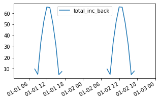
The plot above shows that we’re getting the same results we obtained in the previous tutorial section with the new report generating function.