Getting started

This is a quick overview of multiple capabilities of pvfactors:

• create a PV array

• use the engine to update the PV array

• plot the PV array 2D geometry for a given timestamp index

• run a timeseries bifacial simulation using the “full mode”

• run a timeseries bifacial simulation using the “fast mode”

Imports and settings

# Import external libraries
import numpy as np
import matplotlib.pyplot as plt
from datetime import datetime
import pandas as pd
import warnings
warnings.filterwarnings("ignore", category=RuntimeWarning)

# Settings
%matplotlib inline
np.set_printoptions(precision=3, linewidth=300)

Get timeseries inputs

df_inputs = pd.DataFrame(
    {'solar_zenith': [20., 50.],
     'solar_azimuth': [110., 250.],
     'surface_tilt': [10., 20.],
     'surface_azimuth': [90., 270.],
     'dni': [1000., 900.],
     'dhi': [50., 100.],
     'albedo': [0.2, 0.2]},
    index=[datetime(2017, 8, 31, 11), datetime(2017, 8, 31, 15)]
)
df_inputs

	solar_zenith	solar_azimuth	surface_tilt	surface_azimuth	dni	dhi	albedo
2017-08-31 11:00:00	20.0	110.0	10.0	90.0	1000.0	50.0	0.2
2017-08-31 15:00:00	50.0	250.0	20.0	270.0	900.0	100.0	0.2

Prepare some PV array parameters

pvarray_parameters = {
    'n_pvrows': 3,            # number of pv rows
    'pvrow_height': 1,        # height of pvrows (measured at center / torque tube)
    'pvrow_width': 1,         # width of pvrows
    'axis_azimuth': 0.,       # azimuth angle of rotation axis
    'gcr': 0.4,               # ground coverage ratio
}

Create a PV array and update it with the engine

Use the PVEngine and the OrderedPVArray to run simulations

from pvfactors.engine import PVEngine
from pvfactors.geometry import OrderedPVArray

# Create an ordered PV array
pvarray = OrderedPVArray.init_from_dict(pvarray_parameters)
# Create engine using the PV array
engine = PVEngine(pvarray)
# Fit engine to data: which will update the pvarray object as well
engine.fit(df_inputs.index, df_inputs.dni, df_inputs.dhi,
           df_inputs.solar_zenith, df_inputs.solar_azimuth,
           df_inputs.surface_tilt, df_inputs.surface_azimuth,
           df_inputs.albedo)

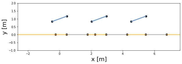
The user can then plot the PV array 2D geometry for any of the simulation timestamp

# Plot pvarray shapely geometries
f, ax = plt.subplots(figsize=(10, 3))
pvarray.plot_at_idx(1, ax)
plt.show()

Run simulation using the full mode

The “full mode” allows the user to run the irradiance calculations by accounting for the equilibrium of reflections between all the surfaces in the system. So it is more precise than the “fast mode”, and it happens to be almost as fast.

# Create a function that will build a report from the simulation and return the
# incident irradiance on the back surface of the middle PV row
def fn_report(pvarray): return pd.DataFrame({'qinc_back': pvarray.ts_pvrows[1].back.get_param_weighted('qinc')})

# Run full mode simulation
report = engine.run_full_mode(fn_build_report=fn_report)

# Print results (report is defined by report function passed by user)
df_report_full = report.assign(timestamps=df_inputs.index).set_index('timestamps')

print('Incident irradiance on back surface of middle PV row: \n')
df_report_full

Incident irradiance on back surface of middle PV row:

	qinc_back
timestamps
2017-08-31 11:00:00	106.627832
2017-08-31 15:00:00	79.668878

Run simulation using the fast mode

The “fast mode” allows the user to get slightly faster but less accurate results for the incident irradiance on the back surface of a single PV row. It assumes that the incident irradiance values on surfaces other than back surfaces are known (e.g. from the Perez transposition model).

# Run the fast mode calculation on the middle PV row: use the same report function as previously
df_report_fast = engine.run_fast_mode(fn_build_report=fn_report, pvrow_index=1)

# Print the results
print('Incident irradiance on back surface of middle PV row: \n')
df_report_fast

Incident irradiance on back surface of middle PV row:

	qinc_back
2017-08-31 11:00:00	107.934226
2017-08-31 15:00:00	83.495861

We can observe here some differences between the fast and full modes for the back surface total irradiance, which are mainly due to the difference in how reflections are accounted for.