View Factors

Theory

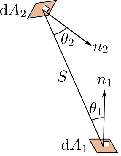
The view factors, also called configuration factors, come from the definition of the directional spectral radiative power of a differential area.

Let’s take the example of black body surfaces, and then extrapolate the results to more general ones.

For a black body differential area \(dA_1\), we can write that the radiative power emitted to another black body differential area \(dA_2\) is:

\[d^2 Q_{{\lambda}, d1-d2}{\;}d{\lambda} = i_{{\lambda},b,1}{\;}d{\lambda}{\;}d{\omega}_1{\;}dA_{1, projected}\]

where:

* \(d^2 Q_{{\lambda}, d1-d2}\) is the spectral radiative power from \(dA_1\) to \(dA_2\)

* \(i_{{\lambda},b,1}\) is the blackbody spectral intensity from \(dA_1\)

* \({\lambda}\) is the wavelength

* \(d{\omega}_1\) is the solid angle from \(dA_1\) to \(dA_2\)

* \(dA_{1, projected}\) is the projected area \(dA_1\) onto the S direction

We can then integrate over \({\lambda}\) for a black body and rearrange:

\[d^2 Q_{d1-d2}{\;} = {\frac{{\sigma}{\;}T_1^4}{{\pi}}}{\;}d{\omega}_1{\;}cos{\theta}_1{\;}dA_1\]

Then:

\[d^2 Q_{d1-d2}{\;} = {\frac{{\sigma}{\;}T_1^4}{{\pi}}}{\;}{\frac{cos{\theta}_2{\;}dA_2}{S^2}}{\;}cos{\theta}_1{\;}dA_1\]

And finally:

\[{\frac{d^2 Q_{d1-d2}}{dA_1}} = {\sigma}{\;}T_1^4 {\frac{cos{\theta}_2{\;}cos{\theta}_1}{{\pi}{\;}S^2}}{\;}dA_2\]

The view factor from the differential area \(dA_1\) to the differential area \(dA_2\) is then defined as:

\[d^2F_{d1-d2}{\;} = {\frac{cos{\theta}_2{\;}cos{\theta}_1}{{\pi}{\;}S^2}}{\;}dA_2\]

And for two finite areas \(A_1\) and \(A_2\):

\[F_{1-2}{\;} = {\frac{1}{A_1}}\int_{A_1}\int_{A_2}d^2F_{d1-d2}{\;}dA_1{\;} = {\frac{1}{A_1}}\int_{A_1}\int_{A_2}{\frac{cos{\theta}_2{\;}cos{\theta}_1}{{\pi}{\;}S^2}}{\;}dA_2{\;}dA_1\]

We can also note that by reciprocity:

\[A_1{\;}F_{1-2} = A_2{\;}F_{2-1}\]

This approach also holds for diffuse surfaces, whose optical properties don’t depend on the direction of the rays.

We can understand the view factor from a surface \(A_1\) to a surface \(A_2\) as the fraction of the hemisphere around \(A_1\) that is occupied by \(A_2\).

Application

We will be using configuration factors in the case of 2D geometries, which simplifies the calculations. The 2D assumption is made because the tracker rows considered will be fairly long, and the edge effects will therefore have less impact.

Also, instead of doing the numerical integration of the double integral representing the view factor, we will systematically try to use analytical solutions of those integrals from tables.

Here are links describing some view factors relevant to PV array geometries.

• View factor of a wedge: http://www.thermalradiation.net/sectionc/C-5.html

• View factor of parallel planes: http://www.thermalradiation.net/sectionc/C-2a.htm

• View factor of angled planes: http://www.thermalradiation.net/sectionc/C-5a.html

• The Hottel method is also widely used in the model

Adding non-diffuse reflection losses

For the derivation shown above, we assumed that the surfaces were diffuse. But as shown in 1, it is possible to add an approximation of non-diffuse effects by calculating absorption losses that are function of the angle-of-incidence (AOI) of the light.

If we’re interested in calculating the absorbed irradiance coming from an infinite strip to an infinitesimal surface, we can calculate a view factor derated by AOI losses by starting with the formula derived in http://www.thermalradiation.net/sectionb/B-71.html.

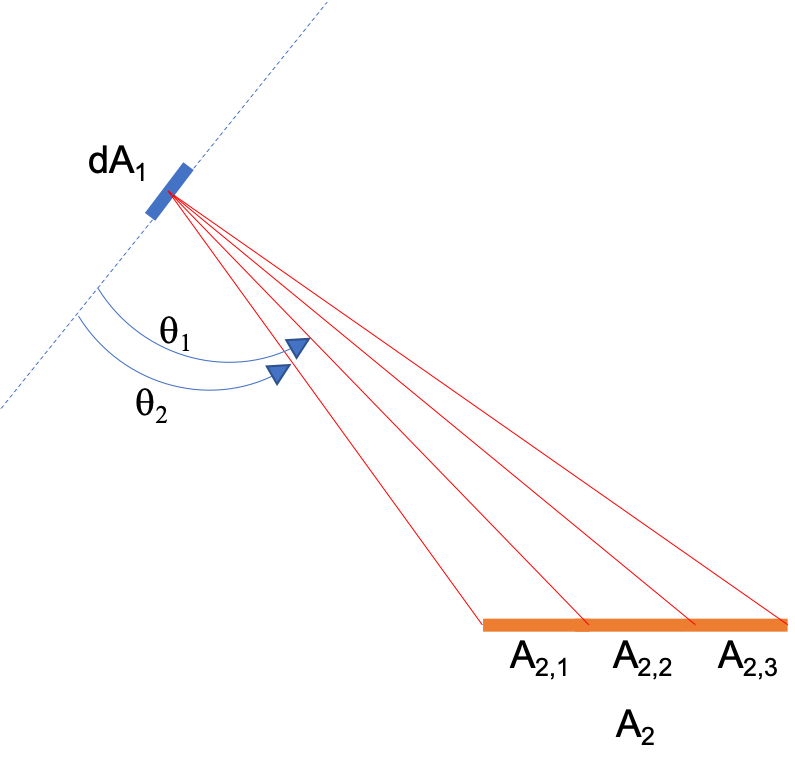
Fig. 1: Schematics illustrating view factor formula from dA1 to infinite strips

The view factor from the infinitesimal surface \(dA_1\) to the infinite strip \(A_{2,1}\) is equal to:

\[dF_{dA_{1}-A_{2,1}}{\;} = {\frac{1}{2}}{\;}({cos{\theta}_2{\;}-{\;}cos{\theta}_1})\]

For this small view of the strip, we can assume that a given AOI modifier function (\(f(AOI)\)), which represents reflection losses, is constant. Such that:

\[dF_{dA_{1}-A_{2,1},AOI}{\;} = {\frac{1}{2}}{\;}f(AOI){\;}({cos{\theta}_2{\;}-{\;}cos{\theta}_1})\]

We can then calculate the view factor derated by AOI losses from the infinitesimal surface \(dA_{1}\) to the whole surface \(A_{2}\) by summing up the values for all the small strips constituting that surface. Such that:

\[dF_{dA_{1}-A_{2},AOI}{\;} = {\sum}_{j=1}^{3}{\;}dF_{dA_{1}-A_{2,j},AOI}\]

Note

Since this formula was derived for “infinitesimal” surfaces, in practice we can cut up the PV row sides into “small” segments to make this approximation more valid.

1

Marion, B., MacAlpine, S., Deline, C., Asgharzadeh, A., Toor, F., Riley, D., Stein, J. and Hansen, C., 2017, June. A practical irradiance model for bifacial PV modules. In 2017 IEEE 44th Photovoltaic Specialist Conference (PVSC) (pp. 1537-1542). IEEE.