Mathematical Model

In order to use the view factors as follows, we need to assume that the surfaces considered are diffuse (lambertian). Which means that their optical properties are independent of the angle of the rays (incident, reflected, or emitted).

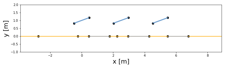
The current version of the view factor model only addresses PV rows that are made out of straight lines (no “dual-tilt” for instance), with a flat ground. But the PV array can have any azimuth or tilt angle for the simulations. Below is the 2D representation of such a PV array, plotted with pvfactors.

The mathematical model used in pvfactors simulations is different depending on the simulation type that is run.

in “full simulations”, all of the reflections between the modeled surfaces are taken into account in the calculations, which leads to results that account for the equilibrium of reflections between surfaces.
in “fast simulations”, assumptions are made on the reflected irradiance from the environment surrounding the surfaces of interest.

Full simulations

When making some assumptions, it is possible to represent the calculation of irradiance terms on each surface with a linear system. The dimension of this system changes depending on the number of surfaces considered. But we can formulate it for the general case of n surfaces.

For a surface i we can write that:

\[q_{o, i} = q_{emitted, i} + q_{reflected, i}\]

Unit: \(W/m^2\).

* \(q_{o, i}\) is the radiosity of surface i, and it represents the outgoing radiative flux from it.
* \(q_{emitted, i}\) is the emitted radiative flux from that surface. For instance the total emitted radiative flux of a blackbody is known to be \({\sigma}T^4\) (with \(T\) the surface temperature and \({\sigma}\) the Stefan–Boltzmann constant).
* \(q_{reflected, i}\) is the reflected flux from that surface.

Finding values of interest like back side irradiance can only be done after finding the radiosity \(q_{o, i}\) of each surface i. This can become a very complex system of equations where one would need to solve the energy balance on the considered systems .

But if we decide to make the assumption that \(q_{emitted, i}\) is negligible, we can simplify the problem in a way that would enable us to find more easily some approximations of the values of interest. For now, this assumption makes some sense because the temperatures of the PV systems and the surroundings are generally not very high (< 330K). Besides the surfaces are not real black bodies, which means that their total (or broadband) emissions and absorptions will be even lower.

Under this assumption, we end up with:

\[q_{o, i}{\;}{\approx}{\;}q_{reflected, i}\]

where:

\[q_{reflected, i} = {\rho_i} * q_{incident, i}\]

with:
* \(q_{incident, i}\) is the incident radiative flux on surface i.
* \({\rho_i}\) is the total reflectivity of surface i.

We can further develop this expression and involve configuration factors as well as irradiance terms as follows:

\[q_{reflected, i} = {\rho_i} * ({\sum_{j} q_{o, j} * F_{i, j}} + Sky_i)\]

where:
* \({\sum_{j} q_{o, j} * F_{i, j}}\) is the contribution of all the surfaces j surrounding i to the incident radiative flux onto surface i.
* \(F_{i, j}\) is the configuration factor (or view factor) of surface i to surface j.
* \(Sky_i\) is a sky irradiance term specific to surface i which contributes to the incident radiative flux  \(q_{incident, i}\), and associated with irradiance terms not represented in the geometrical model. For instance, it will be equal to \(DNI_{POA} + circumsolar_{POA} + horizon_{POA}\) for the front (illuminated) side of the modules, when using the HybridPerezOrdered model.

This results into a linear system that can be written as follows:

\[ \begin{align}\begin{aligned}\mathbf{q_o} = \mathbf{R} . (\mathbf{F} . \mathbf{q_o} + \mathbf{Sky})\\(\mathbf{R}^{-1} - \mathbf{F}).\mathbf{q_o} = \mathbf{Sky}\end{aligned}\end{align} \]

Or, for a system of n surfaces:

\[\begin{split}(\begin{pmatrix} {\rho_1} & 0 & 0 & \cdots & 0\\ 0 & {\rho_2} & 0 & \cdots & 0\\ \vdots & \vdots & \vdots & \ddots & \vdots\\ 0 & 0 & 0 & \cdots & {\rho_n}\\ \end{pmatrix}^{-1} - \begin{pmatrix} F_{1,1} & F_{1,2} & F_{1,3} & \cdots & F_{1,n}\\ F_{2,1} & F_{2,2} & F_{2,3} & \cdots & F_{2,n}\\ \vdots & \vdots & \vdots & \ddots & \vdots\\ F_{n,1} & F_{n,2} & F_{n,3} & \cdots & F_{n,n}\\ \end{pmatrix}). \begin{pmatrix} q_{o, 1}\\ q_{o, 2}\\ \vdots\\ q_{o, n}\\ \end{pmatrix} = \begin{pmatrix} Sky_1\\ Sky_2\\ \vdots\\ Sky_n\\ \end{pmatrix}\end{split}\]

After solving this system and finding all of the radiosities, it is very easy to deduce values of interest like back side or front side incident irradiance.

Fast simulations

In the case of fast simulations and when interested in back side surfaces only, we can make additional assumptions that allow us to calculate the incident irradiance on back side surfaces without solving a linear system of equations.

In the full simulation case, we defined a vector of incident irradiance on all surfaces as follows:

\[\mathbf{q_{inc}} = \mathbf{F} . \mathbf{q_o} + \mathbf{Sky}\]

And we realized that we needed to solve for \(\mathbf{q_o}\) in order to find \(\mathbf{q_{inc}}\). But with the following assumptions, we can find an approximation of \(\mathbf{q_{inc}}\) for back side surfaces without having to solve a linear system of equations:

we can assume that the radiosity of the surfaces is equal to their reflectivity multiplied by the incident irradiance on the surfaces as calculated by the Perez transposition model 1, which only works for front side surfaces. I.e.

\[\mathbf{q_{o}} ≈ \mathbf{R} . \mathbf{q_{perez}}\]

Here, \(\mathbf{q_{perez}}\) can have values equal to zero for back side surfaces, which will lead to a good assumption if the back side surfaces don’t see each other, which is the case in OrderedPVArray.

we can then also reduce the calculation of view factors to the view factors of the back side surfaces of interest, leading to the following:

\[\mathbf{q_{inc-back}} ≈ \mathbf{F_{back}} . \mathbf{R} . \mathbf{q_{perez}} + \mathbf{Sky_{back}}\]

Example

For instance, if we are interested in back side surfaces with indices 3 and 7, this will look like this:

\[\begin{split}\begin{pmatrix} q_{inc, 3}\\ q_{inc, 7}\\ \end{pmatrix} = \begin{pmatrix} F_{3,1} & F_{3,2} & F_{3,3} & \cdots & F_{3,n}\\ F_{7,1} & F_{7,2} & F_{7,3} & \cdots & F_{7,n}\\ \end{pmatrix} . \begin{pmatrix} {\rho_1} & 0 & 0 & \cdots & 0\\ 0 & {\rho_2} & 0 & \cdots & 0\\ \vdots & \vdots & \vdots & \ddots & \vdots\\ 0 & 0 & 0 & \cdots & {\rho_n}\\ \end{pmatrix} . \begin{pmatrix} q_{perez, 1}\\ q_{perez, 2}\\ \vdots\\ q_{perez, n}\\ \end{pmatrix} + \begin{pmatrix} Sky_3\\ Sky_7\\ \end{pmatrix}\end{split}\]

Grouping terms

For each back surface element, we can then group reflection terms that have identical reflectivity and \(\mathbf{q_{perez}}\) terms into something more intuitive:

\[\begin{split}q_{inc-back} &≈ F_{to\ shaded\ ground} . albedo . q_{perez\ shaded\ ground} \\ &+ F_{to\ illuminated\ ground} . albedo . q_{perez\ illuminated\ ground} \\ &+ F_{to\ shaded\ front\ pv\ row} . \rho_{front\ pv\ row} . q_{perez\ front\ shaded\ pv\ row} \\ &+ F_{to\ illuminated\ front\ pv\ row} . \rho_{front\ pv\ row} . q_{perez\ front\ shaded\ pv\ row} \\ &+ F_{to\ sky\ dome} . luminance_{sky\ dome} \\ &+ Sky_{inc-back}\end{split}\]

This form is quite useful because we can then rely on vectorization to calculate back surface incident irradiance quite rapidly.

Footnotes

1: Perez, R., Seals, R., Ineichen, P., Stewart, R. and Menicucci, D., 1987. A new simplified version of the Perez diffuse irradiance model for tilted surfaces. Solar energy, 39(3), pp.221-231.